A Hierarchical Model Incorporating SegmentedRegions and Pixel Descriptors for VideoBackground Subtraction
Shengyong Chen, SeniorMember,IEEE,Jianhua Zhang, Member,IEEE,Youfu Li, SeniorMember,IEEE,and Jianwei Zhang, Member,IEEE
Abstract—Background subtraction is important for detecting moving objects in videos. Currently, there are many approaches to performing background subtraction. However, they usually neglect the fact that the background images consist of different objects whose conditions may change frequently. In this paper, a novel Hierarchical Background Model (HBM) is proposed based on segmented background images. It first segments the background images into several regions by the mean-shift algo-rithm. Then a hierarchical model, which consists of the region models and pixel models, is created. The region model is a kind of approximate Gaussian mixture model extracted from the histogram of a specific region. The pixel model is based on the cooccurrence of image variations described by histograms of oriented gradients of pixels in each region. Benefiting from the background segmentation, the region models and pixel models corresponding to different regions can be set to different parame-ters. The pixel descriptors are calculated only from neighboring pixels belonging to the same object. The experimental results are carried out with a video database to demonstrate the effectiveness, which is applied to both static and dynamic scenes by comparing it with some well-known background subtraction methods.
IndexTerms—Background subtraction, cooccurrence of image variation, region segmentation, hierarchical background model (HBM), pixel model.
I. INTRODUCTION
![]() OREGROUND detection is fundamental in many systems related to video technology [1] [2]. Obtaining the fore-ground by subtracting a background image from the current frame can be achieved by different methods, such as the mixture of Gaussians (MoGs) [3] [4], the kernel density estimation [5] [6], or the cooccurrence of image variations [7]. However, these methods neglect the fact that the background consists of diverse objects and the changes to diverse objects
OREGROUND detection is fundamental in many systems related to video technology [1] [2]. Obtaining the fore-ground by subtracting a background image from the current frame can be achieved by different methods, such as the mixture of Gaussians (MoGs) [3] [4], the kernel density estimation [5] [6], or the cooccurrence of image variations [7]. However, these methods neglect the fact that the background consists of diverse objects and the changes to diverse objects
Manuscript received March 23, 2011; revised July 30, 2011. This work was supported by the Research Grants Council of Hong Kong [CityU118311], the NSFC [61173096, 60870002, R1110679], the DFG German Research Foundation (grant#1247) the International Research Training Group.
Copyright (c) 2011 IEEE. Personal use of this material is permitted. However, permission to use this material for any other purposes must be obtained from the IEEE by sending a request to pubs-permissions@ieee.org.
Shengyong Chen is with the College of Computer Science, Zhejiang University of Technology, 310023 Hangzhou, China. He was a Alexander von Humboldt Fellow at University of Hamburg, Germany. (e-mail: sy@ieee.org).
Jianhua Zhang and Jianwei Zhang are with the Dept of Informatics, University of Hamburg, Germany (e-mail: {jzhang, zhang}@informatik.unihamburg.de)
Youfu Li is with the Dept of Systems Engineering and Engineer-ing Management, City University of Hong Kong, Hong Kong (e-mail: meyfli@cityu.edu.hk).
caused by changes in the conditions are also diverse. For example, when the background involves trees and buildings, the variations of their color caused by illumination changes, and consequently the number of distributions of MoGs may not be the same (Fig. 1). Yet, the variations between edge pixels of trees and buildings may not have cooccurrence. On the other hand, the consistency of the changes in one object is greater than that in different objects. Therefore, if the background is segmented into multi-regions according to some rules, the different regions can be set to different parameters for background models, from which a better performance of background subtraction can be obtained.
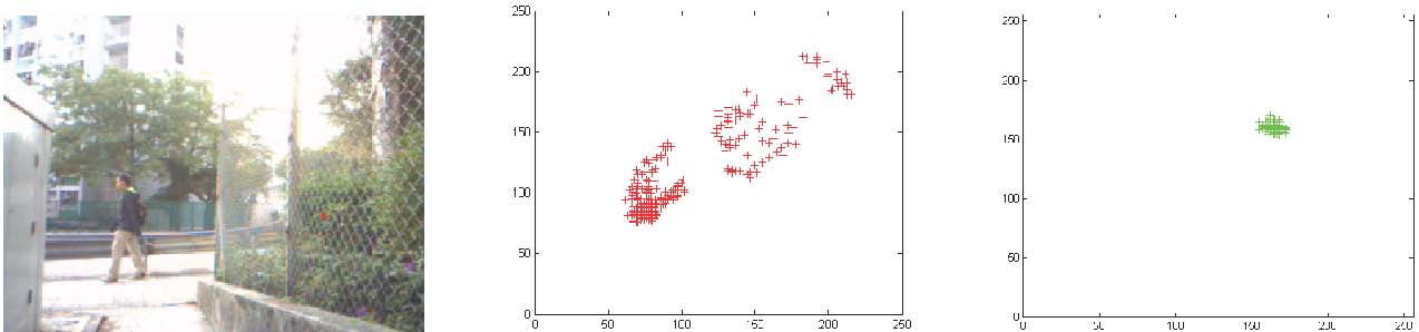
(a) (b) (c)
Fig. 1. Different pixels in the background image and the effect of distributions. (a) Background image. (b) and (c) Scatter plots of the red and green values of a pixel from the image over time.
In this paper, a novel background subtraction method, called Hierarchical Background Model (HBM), is proposed. First, the background images in a training set are segmented by mean-shift segmentation [8]. By using the gray histograms as features, we then build the MoGs with a different number of distributions for each region. The number of distributions can be set manually or computed by an unsupervised cluster algo-rithm (e.g. Affinity Propagation, AP [9]). These MoG models are used as the first level detector to decide which region contains the foreground objects. Next, histograms of oriented gradients of pixels are employed to describe the cooccurrence of image variations within each region. Since the description of cooccurrence is computed by internal pixels in the same region, it can represent the correlation among neighboring pixels more accurately. When updating the model parameters, the rates can also be set separately as the background models are based on regions.
The proposed method is quite different from those existing in the literature using regions and cooccurrence for back-ground subtraction. For instance, in the method proposed by Piccardi and Jan [10], the mean shift is used at the pixel level, while our method employs it to pre-segment the background into different parts. The regions in the method proposed by Varcheie et al. [11] are equal to patches with different sizes. By contrast, the region in our method is one part which is portioned by mean shift and in which there is a certain kind of consistency. Furthermore, by comparison with the one proposed by Wu et al. [12], the region in our method is a kind of dynamic region and can represent the dynamic scene efficiently, while the part mentioned by Wu et al. is a kind of fixed region.
We evaluate the proposed method on the standard test dataset (e.g. CAVIAR, PETS2001 and PETS 2009) and our own test videos. The standard MoGs are used as baseline for comparison. We also compare the proposed method with several state-of-the-art methods that are an effective mixture of Gaussian (EMOG) [4], the background subtraction in [13] in which different parts of the background are modeled by different features (DPDF), the method of effective region based background subtraction (ERB) in [11] and an integrated background model (IBM) in [12]. By comparison with these methods, the main contributions of the proposed method are as follows. First, the hierarchical model can save computing time since the pixel level model is focused on the regions that are detected as containing foreground objects, not on a whole image. Second, by setting different parameters to different regions, complex backgrounds can be modeled by the region-independent parameters in our method. Third, there is stronger consistency within each region since our region is not of regular size but obtained by mean-shift segmentation. Fourth, the borders of regions in our method are dynamically modeled by which the complex dynamic background can be better represented.
II. RELATED CONTRIBUTIONS Background subtraction is a popular method for foreground detection. Many contributions can be found using this tech-nique from different aspects [14] [15]. In [3], Stauffer and Grimson proved the multi-distributional property of pixel values and proposed adaptive background mixture models in
which each pixel is modeled by K-distributions of mixture of Gaussians. An extension of [3] was recently proposed in
[16] by use of a multi-resolution framework. Lee used an adaptive update rate instead of the global and static learning rate to improve the mixture of Gaussians model [4]. However, they all used a fixed number of distributions which cannot adapt to those scenes mentioned above. Recently, in [17] the MoG method is extended to Bayer-pattern image sequences which achieve the same accuracy as MoGs used in RGB color images.
Kernel Density Estimation (KDE) is another frequently-used strategy for background subtraction. Elgammal et al. [5] have proposed a non-parametric model based on KDE from a certain number of the last frames. However, the memory requirement and processing time are high and the bandwidth of kernel estimation is not adaptive. As an improvement for [5], Mittal and Paragios [6] proposed to use an adaptive KDE for background subtraction. However, the consumption of computer resources is still high.
In [7], Seki et al. have exploited the spatial correlation of pixels by using the cooccurrence of image variations. It is an important attempt and they obtained a better performance than other methods where the spatial correlation of pixels is not considered. However, they did not use a more effective strategy to deal with the borders of different background objects which may result in errors.
More recently, some other effective methods have been investigated for background subtraction. For example, Nor-iega and Bernier [18] have employed: i) local kernel color histograms to obtain robust detection against camera noise and little moving objects ii) and contour-based features against illumination changes. Davis and Sharma [19] have developed a method based on contour saliency for background subtraction in thermal imagery. Jung [20] simply makes use of the co-occurrence of pixels in a small area whereas in our method we deal with the co-occurrence of pixels in a more differentiated manner. McHugh et al. [21] use an adaptive threshold to enhance the robustness of their algorithm and also make use of the co-occurrence of pixels in a small spatial neighborhood. Parag et al. [22] have proposed a framework for background subtraction in which different features have been chosen from different regions of background images for modeling corresponding regions. Similarly, the proposed method in this paper also takes into account that the background images consist of multi-regions and different regions have different properties. The method builds the MoGs model for each region segmented by mean shift and makes use of the cooccurrence of pixel variations in the same region to build the models for pixels. We also develop an effective strategy to deal with the borders of different regions.
In [13], a method is presented by taking the discrepancy of parts of background from another perspective, in which different parts are described by different features. However, in this method pixels are only associated to two different types of background objects, stationary and moving ones. Thus pixel changes, given different surroundings, cannot be modeled well. Furthermore, the background is only modeled on the pixel level, which also weakens its performance. Relatively, the proposed method represents the discrepancy of parts of background by setting different parameters for different parts, which can obtain more flexibility for modeling background.
III. OVERVIEW OF THE PROPOSED METHOD
The method proposed in this paper involves two processing levels. The first is for region segmentation obtained by the mean-shift approach [8]. The second is for pixel analysis based on the histogram of oriented gradients. The block diagram of the method is shown in Fig. 2. The first frames of an input video are used to train the model. These frames are segmented into regions by mean-shift. Next, regions in different frames are merged according to their position to form uniform seg-ments for a scene. During this procedure, a dynamic strategy of representing region borders is developed, which leads to a more robust performance for dynamic background. We then compute gray value histograms of these regions to build the region models, and compute the pixel co-occurrence within each region to build the pixel models. The region models are built as Gaussian mixture models with the number of components determined by a cluster algorithm. For detecting foreground objects, we first segment an input frame according to the uniform segments. Next, each region is detected if it contains foreground objects by a corresponding region model. If the detected result shows that a region contains foreground objects, the pixel models are then used to determine which pixel belongs to foreground. After detecting each frame, parameters of region models and pixel models will be updated.
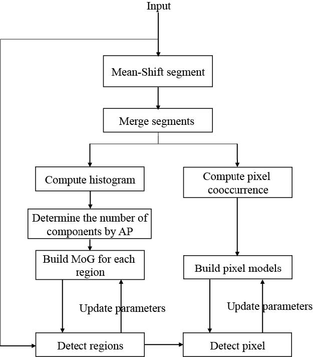
Fig. 2. Block diagram of the proposed method.
IV. REGION MODELS
A. BackgroundImageSegmentation
In this study, we employ the mean-shift approach [23] [24] to segment background images. Although the camera is static, the segmented results still differ among frames since their external conditions change. For example, waving trees and ocean waves can cause changes of the background in dynamic scenes. Even if the background is stationary, the change of the environmental light may also cause different segmentation results. The moving foreground objects also lead to different segments of the backgrounds. When in some frames one part of background is occluded by foreground objects, the segment results are different from other frames where this part is not occluded. Fig. 3 shows the different segmentations between two consecutive frames.
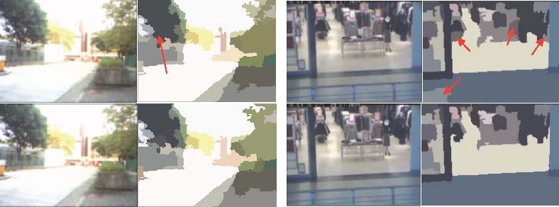
Fig. 3. Different segmenting results of two consecutive frames in a dynamic scene (left), where the regions include waving trees, and a stationary scene (right). The arrows in the top subfigures indicate additional regions that are not in the corresponding bottom subfigures.
However, when a new frame comes, we need to segment it and detect the foreground from its regions. Thus, there must be a unified model which can analyze any new frames using the same rule. Therefore, the segmented results of different background images in the training set must be combined to construct the segmenting model. An algorithm of constructing such a segmenting model is listed in Algorithm 1. Denote:
M: the number of background images for model training;Nu: the number of regions of the u-th background image;RNuk : the k-th region of the u-th background image;S(RNuk ): the area size of RNuk ;
Rk: the k-th unified region;Wk: the pixel weights of the k-th region. Its size is the same
as that of Rk .
Algorithm 1 Pseudocode for unifying the corresponding re-gions.
Require: The threshold indicating the combination of two regions, Ta; Initialization Rk = RN1 k ; Wk(Rk)= 1;
1: for u: from 2 to Mdo
2: for k1: from 1 to N1 do
3: for k2: from 1 to Nudo
u
4: IR = RNk2 ∩ Rk1;
u
5: if S(IR)/S(Rk1 )>Taor S(IR)/S(RNk2 ) > Ta then
6: Rk1 = RNuk2 ∪ Rk1;
7: Update the size of Wk1 equal to new Rk1;
8: Wk1 (IR)=Wk1 (IR)+1;
9: end if
10: end for
11: end for
12: end for
13: for k1: from 1 to N1 − 1 do
14: for k2: from k1 to N1 do
15: IR = Rk1 ∩ Rk2;
16: if S(IR)/S(Rk1 )>Taor S(IR)/S(Rk2 ) > Ta then
17: Rk1 = Rk1 ∪ Rk2;
18: Rk2 =∅;
19: Update the size of Wk1 equal to new Rk1;
20: Wk1 (IR)=Wk1 (IR)+1;
21: end if
22: end for
23: end for
24: Eliminate the empty regions.
At first the algorithm initializes the unified regions to be computed as the regions in the first background image and the weight denotes a pixel belonging to a region as 1. In the first block (line 1 to line 12) the algorithm then computes the intersecting area between each region in the first background image and regions in other background images (line 4). If the intersecting area is larger than a certain threshold, two regions are integrated as one unified region (line 6). At the same time, the weights of pixels in the intersecting area are increased (line 8). By doing this, the regions in different background images corresponding to closed locations will be integrated and the unified regions can be obtained. However, the overlapped areas between adjacent regions may be too large and we need to integrate such regions. In the second block (line 13 to line 24), the algorithm computes the intersected areas among all unified regions (line 15) and integrates regions with the overlapped area larger than a certain threshold (line 17). When a region is integrated into another region, this region will be set to empty (line 18). The weights of pixels in the intersecting area are also increased (line 20). At last, all the empty regions are eliminated (line 24).
After the corresponding regions are merged, we ultimately get the nregions Rk(k ∈ [1,n]). The weight of pixels means the number of their occurrence in one of the ultimate regions over all of the training background images. It can be normalized by dividing it by M. Fig. 4 illustrates the result of final regions in Fig. 3. The left column is the final segment result of two scenes in Fig. 3. The subfigures in the right column are the weighted maps of specific regions pointed out by red arrows. The gray level represents the different weights. The higher gray levels mean larger weights. Because the region in a dynamic scene is not fixed and some pixels on the region border may belong to a different region at another moment, the adjacent regions may overlap.
It was mentioned above that the moving foreground objects will lead to different segments of background. Our method regards those parts of background containing foreground ob-jects as dynamic parts. When building region models, pixels in these parts are assigned weights, just like other dynamic background parts, such as waving trees and waving water.
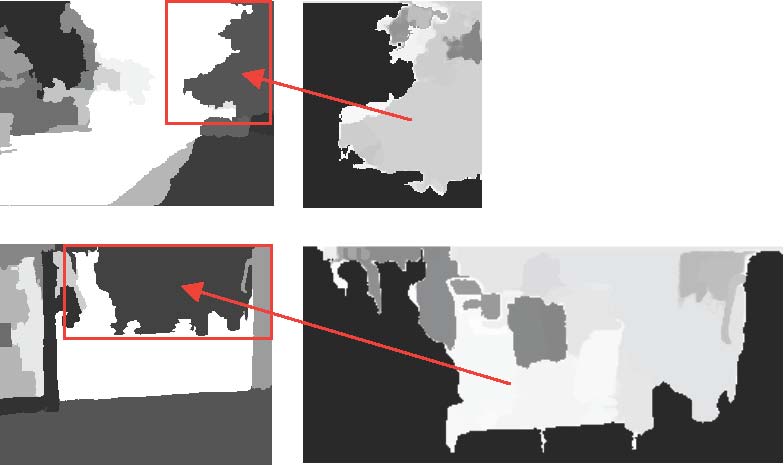
Fig. 4. Region segmentation and pixel weighting.
B. Region Models
Next, the histogram of each region can be calculated ac-cording to the ultimately segmented results. The incrementing addition of each pixel to the corresponding bin of the gray histogram is usually one. However, in the proposed region models, a pixel is not always in the same region. Therefore, for the histogram of each region in each background image, the contribution of a pixel to the corresponding bin is its normalized weight. We can also consider the normalized weight as the probability of this pixel belonging to the region. Hence, we have the following equation to compute the value of the j-th bin in the histogram of the k-th region
hk(j)=K∑Wk(x,y),(p(x,y)∈ bin(j))(1)
where p(x,y)is the pixel value of point (x,y)and bin(j)means the range of pixel values of the j-th bin. Kis a factor which is normalized by the summation of all bin values in the histogram to one. Finally, we obtain Mhistograms for every region. Next, an approximate Gaussian mixture model for each region can be built. In previous contributions [3] [4], the number of distributions of the Gaussian mixture model is a global parameter. It is constant for every pixel in the background. However, constant parameters cannot accurately describe the properties of the changes of each pixel. In the proposed region models, the number of components of each region is different. It can be manually set or obtained from some unsupervised cluster methods. In this paper, we employ the AP cluster method [9] to calculate the number of components. The number of clusters does not need to be determined at first but be computed by the data themselves. By adjusting the ‘preference’ parameter, the number of clusters can be changed to a suitable number. The larger ‘preference’ parameter leads to a larger number of components. Denoting
the Bhattacharyya distance dk = ∑L hni hm between the n-
nmi=1 i
th and m-th histograms of the k-th region (where Lis the number of bins), it can be used to measure the histogram similarity as parameters for input to the AP cluster. The mean of the Bhattacharyya distances of all histograms of the same region, dk, is used as the ‘preference’ parameter of AP. We first choose the most stable region whose number of components can be estimated and then adjust the ‘preference’ parameter by adding a regulating factor γto obtain the satisfactory number of components. Therefore, the ‘preference’ parameter is actually γdk. After we get a suitable γ, the number of distributions of other regions can be computed finally.
Assuming that the number of components of the k-th region is Ck, and the i-th component contains eki entries, we then have the following weight for this component (recall that we used Mbackground images used for training).
wki = eki /M (2)
The Bhattacharyya distances among all entries are used to fit a normal distribution Gki (µik ,σik)and its mean and covariance are denoted as µik and σik .
After fitting the normal distribution for the components of all regions, we obtain the region models. Because these region models take the difference between regions into account, they can more accurately reflect the properties of some dynamic scenes. Moreover, the number of components of models is not a global parameter which could describe the characteristics of different regions.
C. Foreground Detection
To detect the foreground in each region, the current frame is firstly segmented according to the unified segmenting model. After that we compute the histogram for each region. The value of each bin is calculated according to 1. For the histogram of the k-th region of the current frame, the Bhattacharyya distances between the region and the average histogram of all components in this region are computed. Denoting dik as the distance between the current histogram and the i-th component, if it is closer to the mean distance of this component, it is more likely to belong to the background. Therefore, the following equation is used to measure the probability of this region that belongs to the background:
Ck �
pkreg = ∑wki F(dik ,Gik)[1 − F(dik , Gik)] (3)
i=1
where F(dik ,Gki )is the normal cumulative distribution func-tion of dik corresponding to Gki . With the normal distribution, most cases of an instance are within ±3 standard deviations (σ) when the corresponding values of the normal cumulative distribution range from 0.05 to 0.95. Therefore the minimal
k
value of each is � (0.05 × 0.95)=0.22. Because ∑Ck is
i=1 withe sum of weights and equal to 1, the values of preg k for most background regions are larger than 0.22. Note that to use a uni-form threshold for the normal cumulative distribution does not mean the same for the mixture Gaussian distribution. Actually, the threshold related to the mixture Gaussian distribution is adaptive since a histogram of the background region is within 3σand each threshold is different from the others. This is similar to the threshold set in [3] for the standard background Gaussian mixture model where the background pixel value is within 2.5σ. Therefore, with this equation we can set a uniform threshold for all regions to decide whether the region involves foreground or not.
reg ≥ Tr
bgk = 1, pkk (4)
0, preg ≤ Tr
In 4, value ‘1’ signifies that the region is the background and value ‘0’ means that the region contains foreground. The threshold can be set to 0.22.
D. UpdatingParametersinaRegionModel
During the process of updating parameters, one of the most important problems is how to set the updating rate. If the rate is too slow, the model cannot reflect the change of the background in time. On the other hand, if the rate is too fast, it will make the model too sensitive to noise and foreground pixels. Moreover, the manner of updating parameters is another crucial issue. Some methods use a global updating rate. These methods do not take the difference between the background objects’ changes into account. Other methods compute a unique updating rate for every background pixel. However, these methods ignore the consistency of changes of pixels in local regions and make the process very time-consuming.
When segmenting the background into a certain number of regions, the proposed method can overcome these problems by assigning different updating rates to different regions. Thus different region models can be updated separately. The algorithm of updating is similar to [4]. The difference is that the newly proposed model applies a varying update rate while the algorithm in [4] uses a uniform update rate for all pixels. The algorithm for updating model parameters is illustrated in Algorithm 2 where the symbols denote:
n: the number of regions;
αk: the controlling variable for update rates;
ηik: the update rate for the i-th component of the k-th region;NCk: the number of frames detected as foreground for the
k-th region; Ck: the number of components of the Gaussian mixture model of the k-th region; B(H1,H2): the Bhattacharyya distance between histogram H1 and H2;
Hk,ref(t −1): the j-th reference histogram of the k-th region
j
at time (t− 1);
µik ,σik: the parameters of the i-th component of the Gaussian mixture model in the k-th region;
cik: the counter for accumulating the number of matches to the i-th component of the Gaussian mixture model in the k-th region.
Algorithm 2 Pseudocode for updating parameters of region models.
Require: Control variables: n,αk ,TNC; Initialization NCk =0; cki = 0;
1: for each region k: from 1 to ndo
2: Calculate Hk,currthe histogram of k-th region;
3: ∀ j=1Ck ,dkj ,curr=B(Hk,curr, Hkj ,ref(t − 1));
···
4: if region kdoes not involve foreground then
5: NCk = 0;
6: else
7: NCk = NCk +1; Record the histogram of this region;
8: end if
9: for i: from 1 to Ck do
k 1,if i=argmaxj(dkj ,curr)
10: qi = ;0, otherwise
11: wik(t)=(1 − αk)wik(t − 1)+αkqki ;
12: if qik >0 then
k
13: cki = cki + qki ; ηik = qki ( 1−ci αk + αk);
14: Hk,ref(t)=(1 − ηik)Hk,ref(t − 1)+ηikHk,curr;
j jj
15: µik(t)=(1 − ηik)µik(t − 1)+ηikdk,curr;
i
16: (σik(t))2 =(1 − ηik)(σik(t − 1))2 + ηik(dk,curr−
i µik(t − 1))2;
17: end if
18: end for
19: if NCk >TNCthen
20: ∀ j=1Ck ,wkj =(1 − αk)wkj (t − 1);
···
21: i=argminjwj,wj=αk ,cij = 1;
22: Determine other parameters of new components;
23: end if
24: Normalize the weight for each region model;
25: end for
After computing the histograms for each region in a new frame (line 2) and comparing them to the reference histograms to determine which region contains the foreground (line 3), the weight for each component is then updated (line 11) and the most important steps are to compute the update rate (line 13) and to update parameters (line 14-16) according to the update rate. Compared with [3], this algorithm combines fast convergence and temporal adaptability because ηik converges to αk instead of zero and ηik is computed for each Gaussian based on current likelihood estimates in a manner consistent with the incremental EM algorithm. The larger αk leads to a faster update rate and it can be used to those regions which are changed more frequently. How to set αk will be discussed in the experimental section. From line 19 to line 23, we replace an old component with minimal weight in a region model when this region is detected as involving foreground in continuing TNCframes.
V. PIXEL MODELS In pixel models, i.e. the second level of the proposed hierarchy models, we use the spatial correlation between neighboring pixels, which can be immediately proved [14], to describe the pixels. Many approaches have considered this in different manners. The simplest one is the application of binary morphology to refine the results of foreground detection. The formal exploit of the spatial correlation can be found in [7]. However, the border pixels between different objects which have lower
correlation cannot receive the special treatment in [7]. Thus the background subtraction may lead to some wrong results.
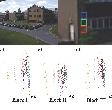
Fig. 5. Distribution of image patterns on block I, II, and III. The point pairs observed within the same time interval are indicated with the same color.
For example, in the top row of Fig. 5, there are three adjacent blocks on different background objects, where block I is on the tree and block II and III are on the building. We com-pute the distributions of image patterns of the three blocks by using the same method as employed in [7]. Since block I and block II are located on different objects, the difference in their distributions is larger than that between block II and block III. Therefore, when the spatial correlation of neighboring pixels is used to describe one pixel, the accuracy can be enhanced by using only the neighboring pixels located on the same object to calculate the spatial correlation. Because we have segmented the background image into different regions, it can be easily implemented to compute the spatial correlation in this manner by taking the neighboring pixels in the same region into account. Furthermore, the spatial correlations used in our pixel model are represented by the Histogram of Oriented Gradient (HOG), which has been proved more robust than that by pixel values or their gradients.
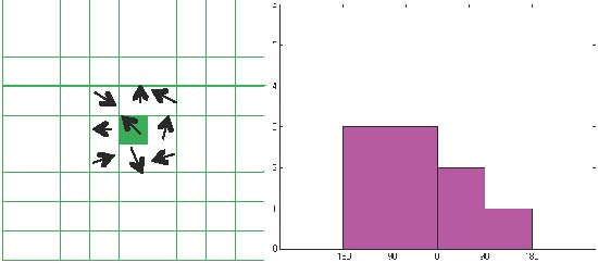
Fig. 6. An example of the histogram of oriented gradients of one pixel.
A. Descriptor of pixels
The pixel descriptor in the proposed method is illustrated in Fig. 6. When the descriptor of one pixel is computed, its 80 neighboring pixels are used and divided into nine blocks where each block consists of nine pixels. In each block, the gradient orientations of all pixels are calculated (such as the left plot in Fig. 6). The orientation (from −πto π) is divided into four bins, which are {[−π,−π/2),[−π/2,0),[0,π/2),[π/2,π)}. Therefore a histogram with four bins for one block is formed (such as the right plot in Fig. 6). Since there are 9 blocks, the histograms of all blocks are combined to form a vector with 36 elements to describe the pixel. It takes the local distributions of pixels into account and obtains more robustness against noises than the values of pixels and their gradients.
When the background images are segmented, a weight is set for each pixel to denote its probability belonging to a region. This weight also needs to be taken into account when we compute the pixel descriptor. The weights of those pixels not belonging to the current region are firstly set to zero and each bin of a histogram of each block is calculated according to
hki (j)=Kik ∑Wk(x,y)m(x,y)(5)
where the coordinates (x,y)∈{(x,y)|θ(x,y)∈ bin(j)}. θ(x,y)and m(x,y)represent the orientation and magnitude of a point at (x,y). The imeans the i-th pixel in the k-th region. bin(j)is the range of orientation of the j-th bin. Kik is a normalized factor of the k-th region which causes the summation of the value of all bins in the histogram to be one. Through this method, the influences of other pixels not belonging to the current region can be avoided. However, as the object whose position is not fixed in background images, the pixel locating at the border may belong to this object at one moment and belong to another object at another moment. Thus, it is inevitable for the calculation of the descriptors of these border pixels to use those pixels which do not belong to the same object. In this case, our method takes the probability of one pixel belonging to the object into account, which can result in a more accurate descriptor.
B. Building Pixel Models
After the descriptors of one pixel over all background images are obtained, the pixel model can be built. Since the descriptor of the pixel is described by the spatial correlation of its neighboring pixels and the change of this pixel is consistent with the change of its neighboring pixels, it is enough to use a unified Gaussian to build the pixel model.
Given Mdescriptors for one pixel obtained from Mback-ground images, the mean descriptor is calculated first. Denote gik as the mean descriptor of the i-th pixel in the k-th region. The Bhattacharyya distances among Mdescriptors of the pixel and gki are then computed. For one pixel (x,y), the unified Gaussian can then be fitted, denoted as PGki (µik(x,y),σik(x,y)). Thus, for one pixel, we have built the pixel model which contains three parameters: gik , µik, and σik .
C. Detection of Foreground
Since the regions involving foreground have been detected by region models, it is unnecessary to use the pixel model to locate the position of the foreground in the whole image, which will significantly reduce the time-cost of detection.
According to the method mentioned in the previous two subsections, the descriptor of one pixel is computed in a new frame. We then compute the Bhattacharyya distance between the current descriptor and the mean descriptor of the corre-sponding pixel model. The probability pik(x,y)of the i-th pixel (x,y)in the k-th region belonging to the background in the new frame can be calculated proportionally by a normal cumula-tive distribution function, F(hki (x,y),PGik(µik(x,y),σik(x,y))), where hki (x,y)means the HOG descriptor of the pixels in the new frame.
pik(j)=F(1 − F) (6)
The computation of this probability is similar to that of the region model. We also set a threshold Tp=0.22 to decide whether the pixel belongs to the background. When pik(x,y)is larger than Tp, pixel (x,y)is claimed to belong to the background. Otherwise, it belongs to the foreground.
However, there are some pixels that may be in two or more intersecting regions. Therefore, the probabilities of these pixels can be calculated as follows
Kp(x,y)=∑ pik(x,y)wik(x,y)(7) k=1
where k=1 to Kimplies that there are Kregions involving the pixel. If the ultimate probability is larger than Tp, the pixel is part of the background.
D. Updating Parameters
We still need a strategy for updating the parameters of the pixel model. Since there are only three parameters for each pixel model, the updating strategy is simpler than that of the region model. Using the same updating method as the region model, the pixel models in different regions are given with different updating rates. They are updated by these rules
gk,ref(t)=(1 − ρik)gk,ref(t − 1)+ρikgk,curr(8)
i ii
µik =(1 − ρik)µik(t − 1)+ρikbki ,curr(9)
(σik(t))2 =(1 − ρik)(σik(t − 1))2 + ρik(bki ,curr− µik(t − 1))2
(10) where ρik = β kPGki (bik,curr|µik(x,y),σik(x,y))is the updating rate controlled by βk that is a constant value to the whole region. If one pixel has been continuously classified as fore-ground for a certain time, this pixel needs to be treated as background. However, the updating strategy may not be able to obtain the new parameters to reflect the change of the background on time. Therefore, the following steps are employed to compensate for the shortage of this strategy:
1. When one pixel is detected as foreground, record its descriptor. And if the pixel was also detected as foreground in the previous frame, increase the amount of a register which is used to record the number of the pixel being foreground and it will be cleared to zero when the pixel is detected as background again.
- If the amount of the register is larger than a threshold TNO, rebuild the pixel model by using those recorded descriptors according to Subsection III-B.
- Clear the amount of the register to zero, and use the new pixel model to detect the foreground in the following frames until another change of background occurs.
VI. EXPERIMENTS
A. Experiments and Parameters
For evaluating the proposed method, extensive experiments have been carried out on six scenes. The first three are the standard test videos, obtained from PETS 2001, PETS 2009 and CAVIAR. The last three are our own test videos with different scenes. The first of our videos is an outdoor scene with waving trees. The second is an indoor scene with the lighted switch on/off. The third is a water scene with waving water. These test videos contain the typical tasks as mentioned in [25].
For each video, the first 60 frames are used to train the model. The backgrounds of all scenes are automatically sepa-rated into 10 to 20 regions according to the scene complexity. Based on these regions, we can build the region models and associated pixel model.
There is a set of initial parameters when we implement the proposed method in a particular application. To set the number of components of region models, we can first manually assign a number, C0, to a stable region, then the cluster algorithm can adjust a scale parameter, γ, to construct a Gaussian mixture model with C0 components for this region. The γcan be used on other region models to cluster an appropriate number of components.
For different regions, corresponding region models and pixel models are set different controlling variables which determine the update rates. Generally, for a region that changes largely and frequently, its region model will have more components and consequently a larger controlling variable is set, which leads to larger updating rates. The larger updating rates then update the model faster, which can result in a more accurate detection. Therefore, we can set the controlling variables for a region model and associated pixel models as proportional to the number of components of this region model. This manner of setting controlling variables further renders the proposed method more adaptive. In practice, the controlling variables are set to αk = βk = Z ×Ck, where αk and βk are the controlling variables for the kth region model and pixels models associated with this region, respectively. Zis a constant denoting the proportion, and Ck is the number of this region model. In all of our experiments, Zis equal to 0.005.
The threshold TNCis set to 180, which means that a new component can replace an old component if a region contains foreground in 180 consecutive frames. The threshold TNOis set to 60, which means that the background object shifts to another at a pixel if it has been detected as foreground in 60 consecutive frames. TNCand TNOneed to be set for replacing a component of a region model or shifting a pixel model, which only happens when a region or a pixel is detected as foreground over a certain time. Furthermore, before replacing a component of a region model and shifting a pixel model, if a foreground object enters the scene and stays there for a long period, it is regarded as a background object. The proposed method will detect this object as foreground until a new component or a new pixel model is generated. This will not influence the performance of detecting foreground because this object will be detected as a static foreground during this period and the extra cost of the next task for tracking this static object will not be increased too much. After this period, the old component of the region model and the old pixel model will be replaced and this object will be regarded as a background object.
Moreover, we compare the proposed HBM to several state-of-the-art methods as mentioned in Introduction (i.e. EMOG [4], DPDF [13], ERB [11] and IBM [12]), and a standard method (i.e. MOG [3]) as the baseline.
B. Qualitative Evaluation
In Fig. 7, six examples of foreground detection correspond-ing to six test videos are shown. The top row is the result of CAVIAR, which is an indoor scene. Because it is a relatively simple scene, most of the methods obtain good results, except for the DPDF method. The second and third rows are the results of PETS 2001 and 2009. These two examples are outdoor scenes. Because of the sunlight changes and waving trees, the MOG and EMOG methods obtain relatively poor results. The ERB and IBM methods obtain good results in PETS 2001, while in the PETS 2009 scene, some moving background objects, such as waving trees, result in much inaccurate detection. As it is not sensitive to small foreground objects, the DPDF method cannot correctly detect in the PETS 2001 scene and discards some foreground objects in the PETS 2009 scene. At last it is obvious that the proposed method obtains promising results in all of three scenes.
The fourth row is the result of an indoor scene with light changes. The original picture shows a frame where the light is just switched on. Because of the light changing sharply, those reference methods cannot achieve satisfactory results, while our method obtains the best result with only failure detection occurring in the region of a cabinet. Other regions, such as the door and table regions, where light reflection causes failed detection in the other methods, have been discard by our region models. The fifth row is the result of an outdoor scene with waving trees. Except for the MOG method, most reference methods and our method achieve good results. The last row shows the result of a challenging scene with continuously and randomly changing waving water caused by the moving machine fish. For those reference methods, many failure detections can be found near the water surface. Because the machine fish moves randomly, these methods cannot obtain a complete fish shape. The proposed method uses a dynamic border representation, therefore, there are very few failure detections near the water surface. Moreover, the use of pixel co-occurrence results in a more complete fish shape.
C. Quantitative Evaluation
Now we further give the quantitative experimental results. We compute the ratio of falsely detected foreground according
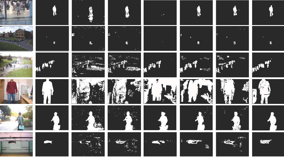
Fig. 7. Results of foreground detection from six test videos. From top to bottom, these videos are from CAVIAR, PETS 2001 and PETS 2009 (resized to 640 × 480) and our own videos, an indoor scene with the light switched on/off, an outdoor scene with waving trees and an waving water scene (320×240). Form left to right, the subfigures are original frames, ground truth, the results of MOG, EMOG, DPDF, ERB, IBM and our method, respectively.
TABLE ITHE RATIOS OF ERROR DETECTION FOR ALL METHODS IN SIX SCENES.
| CAVIAR | PETS ’01 | PETS ’09 | ||||
|---|---|---|---|---|---|---|
| m | var | m | var | m | var | |
| MOG | 0.42 | 0.37 | 0.48 | 0.41 | 0.52 | 0.43 |
| EMOG | 0.39 | 0.25 | 0.43 | 0.24 | 0.48 | 0.37 |
| DPDF | 0.28 | 0.31 | 0.33 | 0.23 | 0.37 | 0.25 |
| ERB | 0.31 | 0.26 | 0.35 | 0.24 | 0.43 | 0.28 |
| IBM | 0.33 | 0.22 | 0.36 | 0.29 | 0.39 | 0.25 |
| HBM | 0.25 | 0.23 | 0.32 | 0.30 | 0.39 | 0.27 |
| Indoor | Outdoor | Water | ||||
| MOG | 0.50 | 0.49 | 0.47 | 0.39 | 0.62 | 0.58 |
| EMOG | 0.42 | 0.42 | 0.49 | 0.28 | 0.56 | 0.49 |
| DPDF | 0.32 | 0.33 | 0.27 | 0.23 | 0.35 | 0.29 |
| ERB | 0.36 | 0.35 | 0.27 | 0.29 | 0.40 | 0.33 |
| IBM | 0.33 | 0.29 | 0.31 | 0.24 | 0.37 | 0.31 |
| HBM | 0.30 | 0.26 | 0.28 | 0.24 | 0.32 | 0.27 |
to the following equation:
err = ∑|Frxd ,y − Frg |/∑Frg (11)
x,yx,y
where the value of Frxd ,y is 1 if pixel (x,y)is detected as foreground and 0 if pixel (x,y)is detected as background. Frxg ,yindicates the ground truth of a pixel depending on whether it is background (the value is 0) or foreground (the value is 1). If the detected result is close to the ground truth, the value of ∑|Frxd ,y − Frxg ,y| trends to 0 and consequently the value of errwill be also close to 0. On the other hand, a large value of ∑|Frxd ,y − Frxg ,y| will result in a large err, which means a poor result of foreground detection. Thus the performance can be evaluated by 11. In the experiments, the ratio of error foreground detection is computed for each frame of all scenes. The mean ratios and corresponding variances for all methods applied in all six scenes are listed in Table I where ‘m’ and ‘var’ denote the means and variances of the ratios. As it can be seen from the table, in most scenes our method achieves the best performance. Although in two scenes, the DPDF method achieves the best results, the ratios of our method are very close to the best ratios.
For the evaluation of the performance of different algo-rithms, the processing rates (fps) for the six methods are listed in Table II. These algorithms are implemented on a personal
TABLE IITABLE IV
COMPARISON OF PROCESSING RATES OF DIFFERENT BACKGROUND THE AVERAGE TIME COST IN THE DETECTION STAGE FOR SIX TESTSUBTRACTION METHODS. VIDEOS (IN MILLISECONDS)
| Resolution | MoG | EMoG | DPDF | ERB | IBM | HBM |
|---|---|---|---|---|---|---|
| 640 × 480 | 8.12 | 8.14 | 7.33 | 8.64 | 8.77 | 9.21 |
| 320 × 240 | 19.21 | 19.02 | 18.65 | 11.06 | 19.67 | 21.27 |
| Test Video | Region Model Detection(ms) | Pixel Model Detection(ms) | Region Number |
|---|---|---|---|
| CAVIAR | 25 | 82 | 15 |
| PETS2001 | 29 | 76 | 16 |
| PETS2009 | 30 | 72 | 16 |
| Indoor | 13 | 24 | 17 |
| Outdoor | 11 | 23 | 14 |
| Water | 19 | 28 | 20 |
TABLE III
THE AVERAGE TIME COST IN THE TRAINING STAGE FOR SIX TEST VIDEOS (IN SECONDS)
| Test Video | Segment Frames | Merge Regions | Train Region Models | Train Pixel Models |
|---|---|---|---|---|
| CAVIAR | 0.042 | 0.423 | 1.9 | 3.2 |
| PETS2001 | 0.048 | 0.465 | 2.1 | 2.9 |
| PETS2009 | 0.051 | 0.509 | 2.2 | 2.7 |
| Indoor | 0.046 | 0.407 | 1.8 | 3.0 |
| Outdoor | 0.050 | 0.450 | 2.1 | 3.1 |
| Water | 0.056 | 0.546 | 2.5 | 3.2 |
computer with a 1.87 Hz Intel Pentium Dual CPU and 2 GB RAM memory, using C++ with OpenCV. As shown in the table, we evaluate the algorithms in different sizes of test videos.
To further analyze the complexity of the proposed method, we investigate the time cost in each phase for model training and foreground detection. In the training stage, four phases are segmenting frames, merging regions, training region models and pixel models. Because using mean-shift to segment a large image is a time-consuming task, all frames are resized to 160 × 120. Thus the average time for segmenting a frame ranges from 0.042 -0.056 seconds for all six scenes. The operation of merging regions is also based on these resized frames to save time. This phase only executes once in the training stage. According to algorithm 1, its complexity is O((M+1)× N¯2), which takes about 0.5 seconds in our experiments. Here Mdenotes the number of training frames and N¯is the average number of segments of all training frames. For training region models, the gray histograms for all regions need to be computed, then an AP cluster algorithm used to obtain the number of components. Since these two algorithms are very fast, this phase takes a short time. The phase of training pixel models has the same situation as the last phase. Thus only a few seconds are needed for the training stage. In Table III the detailed time cost for each phase in this stage is listed. Note that the number in the second column means the average time cost for segmenting each training frame which is processed once for each frame.
In the foreground detection stage, since our method first detects the regions and will ignore the regions without back-ground, the time-cost is decreased. There are two main stages,
i.e. detection of the region model and detection of the pixel model. The average processing times are listed in Table IV for each test video. A larger number of regions will cause a longer processing time of the region model, but the average number of pixels in each region is lower and consequently the processing time of the pixel model is shorter. Note that in this table the time cost in the first three rows is larger than that in the last three rows because the video sizes of the former are larger than those of the latter.
VII. CONCLUSION
In this paper, we have proposed a novel hierarchical back-ground model (HBM) based on region segmentation and pixel descriptors to detect and track foreground. Along with the environmental variation, the changes to different objects in the background are different. Therefore, the proposed method first segments the background into different regions and then builds region models and pixel models. Because in some dynamic scenes, the locations of background objects are not fixed, each pixel of the segmented regions is assigned a weight to denote the probability that this pixel belongs to one region. This way, the proposed models have the following advantages: 1) each model can be set different parameters according to the region that it associates, which will lead to a more accurate description than the constant parameters; 2) the weighted pixels in each region make the descriptor of region and pixel (histogram for the region and histogram of the oriented gradient for pixels) more precise; 3) the hierarchical models which first decide which regions contain foreground and then locate the foreground only in these regions can avoid failing detection in other regions and reduce the time-cost. The experimental results show that the proposed method achieves a better performance than other well-known methods.
REFERENCES
[1] Y. Chen, B. Wu, H. Huang and C. Fan, ”A Real-time Vision System for Nighttime Vehicle Detection and Traffic Surveillance,” IEEETrans.IndustrialElectronics, in press.
[2] B. Armstrong and S. Puthan Veettil, ”Soft Synchronization: Synchro-nization for Network-Connected Machine Vision Systems”, IEEETrans.IndustrialInformatics, vol. 3, no. 4, pp. 263 -274, 2007.
[3] C. Stauffer and W.E.L. Grimson, ”Adaptive background mixture models for real-time tracking,” in Proc.IEEEInt.Conf.onComput.Vis,PatternRecog.1999, June 1999, pp. 246-252.
[4] D.S. Lee, ”Effective Gaussian Mixture Learning for Video Background Subtraction,” IEEETrans.PatternAnal.Mach.Intell.,, vol. 27, no.5, pp. 827-832, 2005.
[5] A. Elgammal, D. Harwood and L.S. Davis, ”Non-parametric model for background subtraction,” in Proc.Euro.Conf.Comput.Vis.2000, June 2000, pp. 751-767.
[6] A. Mittal and N. Paragios, ”Motion-Based Background Subtraction Using Adaptive Kernel Density Estimation,” in Proc.IEEEConf.onComput.Vis.PatternRecog., 2004, pp.302-309.
[7] M. Seki, T. Wada, H. Fujiwara and K. Sumi, ”Background subtraction based on cooccurrence of image variations,” in Proc.IEEEConf.onComput.Vis.PatternRecog., 2003, vol. 2, pp. 65-72.
[8] D. Comaniciu and P. Meer, ”Robust analysis of feature spaces: color image segmentation,” in Proc.IEEEConf.onComput.Vis.PatternRecog., 1997, pp.750-755.
[9] B.J. Frey and D. Dueck, ”Clustering by Passing Messages Between Data Points,” Science, vol. 315, pp. 972-976, 2007.
[10] M. Piccardi and T. Jan, ”Mean-Shift Background Image Modelling,” in Proc.Int.Conf.ImageProcessing, 2004, vol. 5, pp. 3399-3402.
[11] P. Varcheie, M. S. Lavoie and G. A. Bilodeau, ”An Efficient Region-Based Background Subtraction Technique,” in Proc.CanadianConf.Comput.RobotVis., 2008, pp. 71-78.
[12] W.Hu, H. Gong, S. Zhu and Y. Wang, ”An Integrated Background Model for Video Surveillance Based on Primal Sketch and 3D Scene Geometry,” in Proc.IEEEConf.onComput.Vis.PatternRecog., 2008, pp. 1-8.
[13] L. Li, W. Huang, I.Y.H. Gu and Q. Tian, ”Foreground Object Detection from Videos Containing Complex Background,” in Proc.11thACMInt.Conf.MM, 2003, pp. 2-10.
[14] M. Piccardi, ”Background subtraction techniques: a review,”in Proc.IEEEInt.Conf.Systems,ManandCybernetics, 2004, vol. 4, pp. 3099-3104.
[15] A. Bayona, J. C. SanMiguel and J. M. Martnez, ”Comparative evaluation of stationary foreground object detection algorithms based on background subtraction techniques”, in Proc.6thInt.Conf.AdvancedVideoandSignalBasedSurveillance, 2009, pp. 25-30.
[16] B. Zhong, S. Liu, H. Yao and B. Zhang, ”Multi-Resolution Background Subtraction for Dynamic Scenes,” in Proc.Int.Conf.ImageProcessing, 2009, pp. 3193-3196.
[17] J.K. Suhr,H.G. Jung, G. Li and J. kim, ”Mixture of Gaussians-Based Background Subtraction for Bayer-Pattern Image Sequences,” IEEETrans.CircuitsandSystemforVideoTechnology, vol.21, no.3, pp.365-370, March 2011.
[18] P.Noriega and O. Bernier, ”Real Time Illumination Invariant Back-ground Subtraction Using Local Kernel Histograms”, Proc.BritishMa-chineVis.Conf., 2006, pp. 315-323.
[19] J.W.Davis and V. Sharma, ”Background-Subtraction in Thermal Im-agery Using Contour Saliency,” Int.J.ComputerVision, vol.71, no.2, pp. 161-181, 2007.
[20] C. R. Jung, ”Efcient Background Subtraction and Shadow Removal for Monochromatic Video Sequences,” IEEETrans.Multimedia, vol. 11, no. 3, pp. 571-577, 2009.
[21] J. M. McHugh, J. Konrad, V. Saligrama and P. M. Jodoin, ”Foreground-Adaptive Background Subtraction,” IEEESignalProcess.Lett, vol. 16, no. 5, pp. 390-393, 2009.
[22] T.Parag, A. Elgammal and A. Mittal, ”A Framework for Feature Selection for Background Subtraction,” in Proc.IEEEConf.onComput.Vis.PatternRecog., 2006, pp.1916-1923.
[23] P.Vadakkepat, P. Lim, L. C. D. Silva, L. Jing and L. Ling, ”Multi-modal Approach to Human-Face Detection and Tracking,” IEEETrans.IndustrialElectronics, vol.55, no.3, pp.1385-1393, March 2008.
[24] D. Tsai and J. Luo, ”Mean Shift-Based Defect Detection in Multicrys-talline Solar Wafer Surfaces,” IEEETrans.IndustrialInformatics, vol.7, no.1, pp.125-135, February 2011.
[25] K. Toyama, J. Krumm, B. Brumitt and B. Meyers. ”Wallflower: princi-ples and practice of background maintenance.” in Proc.IEEEInt.Conf.Comput.Vis., 1999, vol. 1, pp. 255?61.
 S. Y. Chen (M’01-SM’10) received the Ph.D. degree in computer vision from the Department of Man-ufacturing Engineering and Engineering Manage-ment, City University of Hong Kong, Hong Kong, in 2003. He joined Zhejiang University of Technology in Feb. 2004 where he is currently a Professor in the College of Computer Science. From Aug. 2006 to Aug. 2007, he received a fellowship from the Alexander von Humboldt Foundation of Germany and worked at University of Hamburg, Germany. From Sep. 2008 to Aug. 2009, he worked as a
visiting professor at Imperial College, London, U.K. His research interests include computer vision, 3D modeling, and image processing. Some selected publications and other details can be found at http://www.sychen.com.nu. He has published over 100 scientific papers in international journals and conferences. He was awarded as the Champion in 2003 IEEE Region 10 Student Paper Competition, and was nominated as a finalist candidate for 2004 Hong Kong Young Scientist Award.
 J. H. Zhang (M’11) received the MSc degree in computer vision from the College of Information Engineering, Zhejiang University of Technology in 2009. He is currently pursuing a PhD degree, with be founded by the DFG German Research Founda-tion (grant#1247) ?International Research Training Group CINACS (Cross-modal Interactions in Natu-ral and Artificial Cognitive Systems), at the Institute of Technical Multimodal Systems at the Department of Informatics at the University of Hamburg, Ger-many. During his study, he joined the project, ”Real-
time Three-Dimensional Data Acquisition by Coded Structured Light”, funded by the National Natural Science Foundation of China (NSFC) and Microsoft Asia Research, completed his thesis on ”the Segmentation of Deformable Object Images Based on Active Shape Model and Image Invariant Features”, and applied for four patents.
 Y. F. Li (M’91-SM’01) received the Ph.D. degree in robotics from the Department of Engineering Science, University of Oxford, Oxford, U.K., in 1993. From 1993 to 1995, he was a Postdoctoral Research Associate in the Department of Computer Science, University of Wales, Aberystwyth, U.K. He joined City University of Hong Kong, Hong Kong, in 1995 where he is currently an Associate Professor in the Department of Manufacturing Engineering and Engineering Management. His research interests in-clude robot vision, sensing, and sensor-based control
for robotics. In these areas, he has published over 100 papers in international journals and conferences. He was associate editors of IEEE Transactions on Automation Science and Engineering (T-ASE) and IEEE Robotics and Automation Magazine (IEEE RA).
 Jianwei Zhang (M’92) received both his Bachelor of Engineering (1986, with distinction) and Mas-ter of Engineering (1989) from the Department of Computer Science of Tsinghua University, Beijing, China, and his PhD (1994) at the Institute of Real-Time Computer Systems and Robotics, Department of Computer Science, University of Karlsruhe, Ger-many. Jianwei Zhang is professor and head of TAMS, Department of Informatics, University of Hamburg, Germany. His research interests are mul-timodal information systems, novel sensing devices, cognitive robotics and human-computer communication. In these areas he has published over 250 journal and conference papers, technical reports, four book chapters and two research monographs. He has received several awards, including the IEEE ROMAN Best Paper Award in 2002 and the IEEE AIM Best Paper Award 2008. Dr. Zhang is member of organization committee of numerous international conferences, including some future ones such as IEEE ICRA 2011 Program Co-chair, IEEE MFI2012 General Chair, IROS 2015 General Chair, etc.