?/span>

Abstract?/span>For pearls and other smooth alike lustrous jewels, the apparent shininess is one of the most important factors of beauty. This paper proposes an approach to automatic assessment of spherical surface quality in measure of shininess and smoothness using artificial vision. It traces a light ray emitted by a point source and images the resulting highlight patterns reflected from the surface. Once the reflected ray is observed as a white-clipping level in the camera image, the direction of the incident ray is determined and the specularity is estimated. As the specular exponent is the most important reason of surface shininess, the method proposed can efficiently determine the equivalent index of appearance for quality assessment. The observed highlight spot and specular exponent measurement described in this paper provide a way to measure the shininess and to relate the surface appearance with white clipped image highlights. This is very useful to industrial applications for automatic classification of spherical objects. Both numerical simulations and practical experiments are carried out. Results of objective and subjective comparison show its satisfactory consistency with expert visual inspection. It also demonstrates the feasibility in practical industrial systems.

Index Terms?/span>surface appearance, quality measurement, specular exponent, classification, shininess index, computer vision

I.     INTRODUCTION

ACH pearl has been elaborated by an unique aliving being. Like other smooth lustrous jewels, the apparent shininess is one of the most important factors of beauty. Unfortunately, automation for pearl classification is rarely studied in the literature and there is no method available to assess the appearance and quality of shininess. In the industry, many characteristics may affect pearl’s quality, but their assessment and classification are still done mostly by human intuitive judgments with very expertised experience.

On the other hand, the recent developed artificial vision technology, which simulates the subjective perception of human inspector [1], provides a convenient way for automatic classification [2]. Many practical applications in robot vision and inspection require interpretation of images of specular, or shiny, surfaces where the perceived brightness becomes a very strong function of viewing direction due to highlights or reflections from the source [3]. Inspection and handling of machine parts, inspection of the shape of solder joint surfaces, and inspecting surface smoothness of metallic or plastic sheets are examples of industrial tasks where surface specularity is a primary consideration [4]. The interpretation of surfaces based on the image brightness pattern of one or more images depends intricately on the prior knowledge of surface properties, image geometry, and light conditions. Vision sensing by shape from shading (with single light source), photometric stereo (with multiple light sources), structured lighting techniques, etc., have generally been used to recover three-dimensional (3D) shapes from one or more images [5] - [7].

Surface shininess is a key index in evaluation of some products like pearls and jewels. In fact, surface shininess is related with its roughness and specularity [8], which have mostly been affecting the function and reliability in industrial components [9]. In the literature, it is well known that different kinds of techniques and methods are used in modeling and measurement of surface roughness [10]. It has been assessed by the judgment of the inspector either by eye or even fingernail. The evaluation was done by comparing the surface to be measured with a standard surface. For an example of surface modeling and image synthesis, Baba proposed a method to model roughness as bump parameters using Gaussian distribution functions [15]. A modern typical surface measuring instrument will consist of a stylus with a small tip (diamond) gauge or transducer, a traverse datum and a processor. The surface is measured by moving the stylus across the surface. Among the mostly used techniques on surface measurement, digital photogrammetry with its measurement sensitivity, practicability, functionality and cost taken together is appealing to users [12].

This paper proposes an idea of automatic evaluation of pearls or pearl-like objects by observation of their surface appearance and physical factors using artificial vision. In the industry, for examining a pearl some basic characteristics, such as the pearl type, size, color and shape, can be determined easily but the work is tedious and laborious. Advanced evaluation may be made on its brightness and surface, as well as the homogeneity of the threads. Numerous factors give rise of its classification, but they do not directly determine the quality. In practice, one factor, called shininess, may much affect the authenticity and beauty of pearls.

In the literature, few attempts have been carried out for pearl evaluation. Nagata, Dobashi, etc. are ones who made early investigation of pearl appearance [13][14]. For modeling and visualization of an evaluation simulator, they proposed an "analysis by synthesis" approach to finding the optimum inspection conditions and inspection criteria through the simulation of the item [13]. An alternative method is carried out by physics-based modeling of internal blurring in the multilayer of a pearl and the partial coherent interference model [14]. Recently, Tian proposed a computer vision-based method for pearl quality assessment [15]. The color is the only feature considered for pearl classification. Images are transformed into HSV (Hue, Saturation, and Value) color space and Fuzzy C-means Clustering Algorithm is used for the classification of pearl saturation. More intensive review for the background can be found in [13]. This system in this paper is vision-based automatic mechatronic system [16] for pearl classification [17]. The algorithm presented uses highlight principle in artificial vision and digital photogrammetry to extract surface light properties. It combines advantages of both photogrammetry and vision perception [18].

The rest of the paper is organized as follows. In Section II, an automatic industrial system is introduced with vision assessment. The formulation of specularity in the vision system with lighting technology is described in Section III. Detailed theoretical method for apparent shininess assessment is developed in Section IV. Experiments are described in Section V and results are discussed. Finally, a conclusion is drawn in Section VI.

II.    
Automatic Assessment System

In design of the mechanical system for automatic pearl inspection and classification [19], we have several principles: (1) during the whole classification process, it is desired to use compressed air for pearl motion driven so that the pearl surface will not be stained or worn; (2) to improve the productivity, we may use a schooling pattern for quality evaluation; (3) for the reasons of manufacturing cost and system maintenance, the equipment is designed in modular structures; and (4) the system should be reconfigurable for different purposes of evaluation or classification. By these considerations, the system is designed as in Fig. 1.

In mechanism, the equipment consists of three sub-systems, i.e. mechanical, air driven, and controlling. A pearl will pass three workspaces for feeding, inspection, and classified separation. The inspection station has a closed box where a point light source and a vision camera are placed, as illustrated at right side in Fig. 1. The system works in following operational principles.

(1) Unclassified pearls are controlled to flow into a micro-vibration device and become a single layer. A plate with a matrix of fixed positions is used to suck up a number of arranged pearls. Each pearl is attached to one elementary hole by negative pressure.

(2) The matrix plate is moved to the inspection station. Each pearl can be rotated there and six images are taken to observe the pearl surfaces from all views. A vision processing procedure is carried out for analysis of the quality of the pearls with these images. In this implementation example, the pearl diameter can vary from 3 mm to 15 mm. Each time it can inspect 100 pearls simultaneously.

(3) The matrix plate is further moved to a separation station where pearls are sent to different output collections according to the classification results.

 

TABLE I?Working phases of the pearl classification system

 

 

 

Fig. 2  Classification for object size, shape, color, and blemish

 

(a)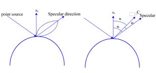

(b)

Fig. 3  Specular exponent and surface shininess. (a) The specularity on smooth surfaces; (b) index of specular exponents (n=40, 20, 10, 5), large number corresponding to finer surface.

 

The pearl classification system consists of five phases in a period, which includes functions of pearl feeding, imaging, orienting, vision processing, and separating. Table I illustrates the working cycle of these phases. On the continuous working line, since phases 1-3 are overlapped with 4 and 5. It can be seen that the period is dominated by the latter, i.e. time = 2.5+5 = 7.5 seconds on the line of one side. The productivity in this example is 13.3 pieces per second (pps).

As can be seen in Fig. 1, the system consists of two working groups that can improve the productivity to double. Its function of classification can be executed according to five evaluation characteristics, including diameter, shape type, color, blemish, and shininess. The former four can be directly determined from the pearl images as illustrated in Fig. 2. In fact, the object size can be determined by d = (D₁ + D₂)/2. D₁ is the maximum diameter, or the longest chord, and it can be determined by finding the maximum distance between any two points on the contour. D₂ is the maximum length of the chords orthogonal to D₁. Regarding the blemish, the pearls are ranked into I, II, III, IV, and V levels according to the flaws detected on the surface. The flaw can be identified in the image according to the color speckle and the level is determined according to the total area size of these speckles. The shape type is classified according to Table II.

 

TABLE II. SHAPE CLASSIFICATION OF PEARLS

* a = (D₁+D₂)/2.

 

TABLE III. COLOR CLASSIFICATION OF PEARLS

 

The pearl color is classified into basic types of white, yellow, purple, although other colors may also be used according to practical requirement. The image is converted into HSV color space and the type is determined by similarity, i.e. the spatial distance in color space, according to Table III.

However, the pearl shininess, one of the most important factors of its beauty, is difficult to be determined directly. In this paper, we utilize the specular exponent of lighting effect as a cue of its appearance quality.

III.     Formulation of Specularity

A.     Specular Surface Reflection

An important class of surface is the glossy or mirror like surface often known as a specular surface [20]. An ideal specular reflector behaves like an ideal mirror. Radiation arriving along a particular direction can leave only along the specular direction, obtained by reflecting the direction of incoming radiation about the surface normal. Usually some fraction of incoming radiation is absorbed; on an ideal specular surface, the same fraction of incoming radiation is absorbed for every direction, the rest leaving along the specular direction [21].

Relatively few surfaces can be approximated as specular reflectors. Typically, unless the material is extremely highly smooth, radiance arriving in one direction leaves in a small lobe of directions around the specular direction. Larger specular lobes mean that the specular image is more heavily distorted and is darker because the incoming radiance must be shared over a larger range of outgoing directions. Quite commonly, it is possible to see only a specular reflection of relatively bright objects like sources. Thus, in some surfaces one sees a bright blob, called specularity, along the specular directions from light sources. We may take the most common Phong model [22], as formulated in (1), to assume that only one point light source is specularly reflected in the inspection system (Fig. 3a).

 

                                                                          ?(1)

 

In this model the radiance leaving a specular surface is proportional to cosⁿq = cosⁿ(q_i - q_s), as in (1), where q_i is the exit angle, i.e. the angle between the surface normal and the observation sight of light, k_s is the specular reflection coefficient, q_s is the specular angle, i.e. the angle between the surface normal and the specular reflection direction, I_ps is point light’s source intensity, I_s is the intensity of the reflection and n is a parameter called specular exponent. Large values of n, which mean surfaces are smooth, lead to a narrow lobe and small sharp specular spot; small values, which mean surfaces are rough, lead to a broad lobe, large specular spot with fuzzy boundaries (Fig. 3b).

B.     Radiometry in the Vision System

From physics and geometry [23], we may find the image irradiance to be

 

                                                                 ??2)

 

where d is the diameter of the lens, a is the angle between the sight of light and the surface normal, and z' is the distance between the image plane and camera optical center.The relationship (2) shows that the object radiance, L, is related to the image irradiance, E, by geometrical factors. We also know that the irradiance is proportional to the area of the lens and inversely proportional to the distance between its center and the image plane.

Considering that in the inspection system the viewing distance to surface points varies very slightly, which means the object radius R is much less than the viewing distance z, i.e. R << z, so that z is approximated as an constant for a pearl, we have L = I_s and a = q_i. Combining (1) and (2) gets (3) or (4)

 

                                     ??3)

                                                            ?4)

 

where a is a constant. The assessment task is to find the index n from the specularity formation (4) by image analysis.

IV.     Assessment Method

A.     Calibration and Measurement

For accurate measurement of different objects, the system has to be calibrated to identify some systematic parameters, e.g. the constants in (3) and (4). Let us firstly consider the light interaction on surfaces. When light interacts with an object, it may be reflected, transmitted, and absorbed. The light reflected from a typical surface in the real world is a combination of the three reflections, i.e. ambient reflection, diffuse reflection, and specular reflection. Ambient reflection is a gross approximation of multiple reflections from indirect light sources. It produces a constant illumination on all surfaces, regardless of their orientation, but itself produces very little realism in images. Diffuse reflection simulates the light that penetrates a surface and gets reflected by the surface in all directions. It is the brightest when the normal vector of surface points toward the light source, but it has nothing to do with the position of the camera. Specular reflection is the direct reflection of light by a surface. Shiny surfaces reflect almost all incident light and therefore have bright specular highlights or hot spots. The location of a highlight moves as you move the camera (view dependent), while keeping the light source and the surface at the stationary position.

In the case of our system setup in Fig. 1, we may assume that there is no ambient reflection in the ideal scene and the surfaces are smooth enough that there is very little diffuse reflection. Therefore, there is only specular reflection considered in closed box of vision inspection. A complete illumination intensity model for reflection from a point light source is shown in (1).

If we choose the roughest surface (seen directly or from a measuring instrument, such as a stylus) and assume n=1, for a scene point near the highlight area we have . Suppose the locations of the point source and the camera are fixed in the inspection box. The coefficient k_s is determined by the surface material and it is changeless when we measure the same kind of objects. From (1), we know that the object radiance E is proportional to image pixel intensity L.

The calibration is necessary for quantitative assessment. If only for qualitative classification of the same kind of objects, we may just take any one to have n = 1 and all others are found relatively smoother or rougher by the assessment method. Referring to the image formation and vision geometry, we can find the relationship between what appears on the image and where it is located in the three-dimensional (3D) world [6].

Suppose we are going to measure some objects whose specular exponents are not yet known. Consider (1) where we keep the same situation as that in the calibration, i.e. source and camera location, the intensity of the source, and we get

 

?/span>,                                   ??5)

 

Therefore, calculation of specular exponent is transformed into seeking the pixel intensity (or gray level) of surface points and corresponding cosq₀. Practically, it still appears hard to carry out, and usually produces inevitable error. In our practice, we use the highlight’s area defined by selecting a certain gray level as threshold value instead.

Consider a smooth surface F(x, y, z) and the normal vector at the incident scene point M(x₀, y₀, z₀) is

 

N_s = [F_x(x₀, y₀, z₀), F_y(x₀, y₀, z₀), F_z(x₀, y₀, z₀)]                             ??6)

 

Assume the coordinates of the light source and the camera are (X_s, Y_s, Z_s) and (X_c, Y_c, Z_c), respectively. By (6), we get the equations where the relationship of incident light and reflected light ray lies

 

,  ??/span>

and     ?/span>                                     ?7)

 

The incident angle q_s is determined by

 

             ??8)

 

The exit angle q_i is determined likewise

 

             ??9)

 

B.     Efficient Calculation Model

The method described in the above subsections is still too complex for practical implementation, especially required for realtime efficiency and system productivity. Now we consider a simplified vision setup and calculation model as illustrated in Fig. 4.

Following the assumptions in Section III, from Fig. 4a the point light source and vision camera are placed at the same position far away from the object. Considering a point on the top area of spherical surface, as R << z, it can be assumed that the line of sight and the incident light are from the same direction to the surface point. According to the geometrical relationship and definitions of viewing and reflecting directions, we have q _s ?/span> -q_i and q ?/span> 2q_i . Therefore, Equation (4) can be rewritten as

 

  

(a)                                               (b)

Fig. 4  Simplified model for specularity calculation on pearl surface. (a) Vision setup and geometrical model; (b) relative calculation of mapped area sizes.

 

       ??10)

 

Let

 

                                                               ??11)

 

where s is highlighted area size and S is the whole size in the great circle, as illustrated in Fig. 4b. We may further get

 

                                                              ?12)

                                                                      ?13)

 

where F = E/a is a constant in (13) which can be determined during the calibration step (when taking the roughest object to have n = 1), i.e.

 

                                                               ??14)

 

Figure 5 plots the relationship between area ratio r_s and spherical shininess n according to (13). It tells that n is rapidly decreasing when r_s is increasing when a rough object is used as a reference. It also means that a “good? object has a small (but very bright) area of highlight. Therefore, the determination of shininess index now becomes easy counting of highlighted pixels. This replacement is very useful for practical implementation because it is actually unlikely to determine the intensity of the central area because of white clipping of the camera.

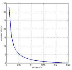
Fig. 5  The shininess index vs area ratio.

 

It should be noted that the paper makes an assumption for the approximation that the pearls have a spherical shape. However, the shape may not always be spherical, but may also ellipsoidal, flat, or irregular as listed in Table II. For different shapes, we can have the same conclusion that the shininess index is related with the highlighted area size. The curves are similar with the one plotted in Fig. 5, but their coefficients are slightly different. For short ellipsoid, there is no problem to evaluate the objects using the same indices, but it may cause a certain error for long ellipsoids and other objects. Fortunately, the pearls are firstly classified by their shapes. Thus the highlighting data can still tell the goodness of pearls well for a same class of pearl shapes. Furthermore, classification of flat and irregular pearls is actually unimportant in the industry.

 

V.     Experiments and Results

A.     Numerical Simulation

To test the validity of the method for determining the specular exponent of a spherical object, we firstly carried out some numerical simulation experiments. From computer vision, we can get the relationship between what appears on the image plane and where it is located in the 3D world [5]. In the simulation, we set some spatial parameters in the world coordinate system. For example of one setup instance, we trace a light ray emitted from the light source at (-3, 3, 3), reflected at a surface point P(0, 0.866, 1.5), and seen by a fixed camera at (0, 10, 1) which images the reflected light ray on the image plane. The image coordinate system is defined with respect to a coordinate system whose origin is at the intersection of the optical axis and the image plane (0,10+λ,1), where λ is the focal length of the camera. From the projective coordinate transformation in computer vision [7], we can easily get the position in the image plane of a scene incident at a point p on the object surface.

In the experiments by means of virtual image generation, when n=1 for the roughest object, we can compute every scene point and generate the virtual image by simulation. It is assumed that the coordinates of the light source, incident scene point and camera are already known. The equation of the sphere is x² + y² + z² = 1. From 3D spatial relationship, we can get the viewing direction cos(q) = 0.96.

By simulation, we assume that λ = 5, the intersection of the optical axis and the image plane is in the image centre. It is assumed n=1 and image attributes are with width 18.6 mm and height 13.1 mm. The actual pixel coordinates (u, v) are numerically determined. In the experiments, the gray level of every image point of P is calculated. The pixel size is with width 0.0322 mm and height 0.0313 mm.

The highlighted area is obtained by pixel summation for those which have the gray levels distributed beyond the white-clipping value, which is 255 for common CCD cameras. However, considering the contrast compression effect, which is used in most cameras, we should set a threshold value on the line of the knee slope. In practice, this paper suggests to use 0.98 of white-clipping value, i.e. 255*0.98=250 in common. A slightly different threshold value does not affect the relative ranking result, but it causes the curve in Fig. 5 shifting a little. Therefore, this value should be consistent in the same task of a ranking application.

Numerically, we change the specular exponents, n, from 1 to 100 and track the highlight reflection fraction with the given point light source. Generated virtual images are shown in Fig. 6. Table IV shows the experimental results of surface shininess measurement from those virtual images. If it is required to obtain the true shininess index, a calibration process should be carried out before its actual measurement. In Table IV, the symbol s represents the highlight area size, which is equivalent to the highlight intensity for a spherical object. The whole ball size is 1540100. The shininess of the first ball is defined to be 1 and the area ratio r_s1 is determined according (11).Then the constant in (14) is found to be F = 0.91. From the results we can find that the measured index N keeps good consistence with the given value. Figure 7 plots the relationship between area ratio r_s and measured index n.

 

 

Fig. 6 ?/span>Virtual images generated for N=1, 2, 4, 8, 10, 20, 30, 50, 80, 100 (from top-left to bottom-right).

 

From Table IV, we can find some difference between the estimated index n and true N. It is mainly caused by the calculation model illustrated in Fig. 4 where we made several approximation assumptions for simplified calculation. Nevertheless, this deviation does not affect the relative relationship between the object shininess and index value. In practice, the measurement is always relative. That is, an object is compared with the one whose index is defined as 1.0. Of course, the deviation can also be corrected by a calibration process which adjusts the curve in Fig. 5 along the true positions.

 

TABLE IV. Measured specular exponents by simulation

 

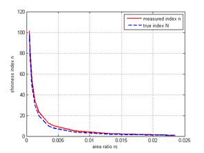
Fig. 7  The shininess index vs area ratio as measured in virtual images.

 

B.     Experiments with real objects

In another experiment, we collect 10 pearls with different appearance quality. The samples are labeled from 1-10 and sorted by experts in a certain order, from worst to best. It means that Pearl No. 1 is worst and No. 10 is best in the sense of shininess. The samples are provided by an industrial company. Since there is no digital criterion available for objective measurement, they are judged by their industrial professional experience.

The images of the sorted pearls are shown in Fig. 8. The same procedure as that of numerical simulation is carried out for pearl assessment and the results are shown in Table V. Without previous calibration, the shininess of the first pearl is defined to be 1 and the area ratio r_s1 is determined according (11). The constant in (14) is found to be F = 0.8625. The pearl size varies somewhat and the equivalent diameters are computed as in the 2nd column in Table V. The highlighted sizes and area ratios are listed in the 3rd and 4th columns. The shininess indices are measured according to (13) and results in listed in the 5th column. The comparison with human visual observation is illustrated in Fig. 9.

Currently, there is no quantitative measurement available for this purpose in the pearl industry. What the experts can tell us is only “which pearl is good/bad?and “which is better/worse? Therefore, we could not give any quantitative comparison, but find the conclusion that the automatic objective assessment is consistent with subjective observation. The research contribution of this paper may provide a new way to quantitative measurement in the industry.

In the experiments, since the assessment procedure only needs to count the number of highlighted pixels in the image and compute the index by (13), the algorithm is very fast (it takes no more than 1 millisecond for each object). Therefore, the method can well meet high efficient requirement of practical applications on real-time production lines.

 

Fig. 8  Images of 10 sample pearls with varying shininess.

 

C.     Discussion

We may notice that although the subjective assessment has a good consistency with the objective observation in general, but is not always identical. From the Fig. 9, we find the shininess indices of the first 3 samples are not monotone increasing. Computer evaluates the shininess index purely according to the light reflection, but human may consider more factors according to individual experience. Especially when the pearls have very similar shininess, it is actually very difficult to tell their difference. Inconsistency may happen in this case, but not always caused by the computer. In fact, it does not require to classify the pearls in such a detailed groups. For example, the industry often uses only three classes, i.e. Class I, II, and III. Therefore, instead of 10, if the pearls are classified into 3 groups, then the result is perfect because the first 3 samples are going to one class.

On the other hand, in the theory we have assumed that only one point source is used for lighting the object, but in the practical design a number of objects are located along each other to improve the productivity. To reduce the reflection effects among them, the light source and the camera are placed on the top of a black box. The light is thus reflected to the top and sides of the box. The black material inside the box can absorb the reflected light from all pearls. The pearls are placed with a certain distance each other to reduce the effect of their reflection. In addition, during image processing for identification of highlighted area, only the top area is computed to avoid noises of the surrounding.  However, this design still can not completely avoid disturbance from each other. A perfect setup is to inspect one pearl in each examination. This can make the result more accurate, but decrease the productivity (to about only 1% of that in the current design). It depends on the interest in the industry. Mostly, it does not need to evaluate very accurately only for classification purpose. The industrial companies only need to separate them into 3 or 4 classes. Of course, in some other applications instead of pearl classification, accurate assessment may still be necessary.

 

Table V. Experimental results of the pearl samples

 

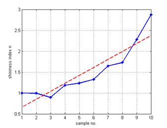
Fig. 9  The shininess indices of 10 sample pearls?(consistency between subjective and objective assessments).

 

VI.     Conclusion

This paper described a novel method to calculate the specular exponent of a surface for assessment of its appearance quality by means of artificial vision. It computes the white-clipped highlight of illumination of a point source and image intensity to observe local surface properties. Since the procedure is mostly to count the number of highlighted pixels in an image, which takes no more than 1 ms for each object, it can produces in very high efficiency in practical applications. Both digital simulation and practical experiments were carried out to test the correctness of the method. The results appear reasonable. The numerical measurement is found correlation with intuitive observation of the appearance. Comparison of subjective and objective matches well. The results obtained so far are promising and provide a basis for the development of a new approach to shininess assessment and automatic inspection systems for classification of pearl-like smooth objects.

References

[1]     M.I. Chacon-Murguia, J.I. Nevarez-Santana, R. Sandoval-Rodriguez, "Multiblob Cosmetic Defect Description/Classification Using a Fuzzy Hierarchical Classifier," IEEE Trans. Industrial Electronics, vol.56, no.4, pp.1292-1299, April 2009.

[2]     A.N. Belbachir, M. Hofstätter, M. Litzenberger, P. Schön, "High-Speed Embedded-Object Analysis Using a Dual-Line Timed-Address-Event Temporal-Contrast Vision Sensor," IEEE Trans. Industrial Electronics, vol.58, no.3, pp.770-783, March 2011.

[3]     G.A. Atkinson, E.R. Hancock, "Recovery of surface orientation from diffuse polarization," IEEE Trans. Image Processing, vol.15, no.6, pp.1653-1664, June 2006.

[4]     S. K. Nayar, et al., “Specular surface inspection using structured highlight and Gaussian images? ?i>IEEE Trans. Robotics and Automation, vol. 6, no. 2, pp.208-218, Apr. 1990.

[5]     Y.-L. Chen, B.-F. Wu, H.-Y. Huang, C.-J. Fan, "A Real-Time Vision System for Nighttime Vehicle Detection and Traffic Surveillance," IEEE Trans. Industrial Electronics, vol.58, no.5, pp.2030-2044, May 2011.

[6]     S. Y. Chen, Y. F. Li, J. Zhang, “Vision Processing for Realtime 3D Data Acquisition Based on Coded Structured Light? IEEE Trans. Image Processing, vol. 17, no. 2, pp. 167-176, Feb. 2008.

[7]     D. G. Aliaga, Y. Xu, "A Self-Calibrating Method for Photogeometric Acquisition of 3D Objects," IEEE Trans. Pattern Analysis and Machine Intelligence, vol.32, no.4, pp.747-754, April 2010.

[8]     B. Kim, W. S. Kim, “Wavelet monitoring of spatial surface roughness for plasma diagnosis? Microelectronic Engineering, vol. 84, no.12, pp. 2810-2816, Dec. 2007.

[9]     F. Immovilli, et al., "Detection of Generalized-Roughness Bearing Fault by Spectral-Kurtosis Energy of Vibration or Current Signals," IEEE Trans. Industrial Electronics, vol.56, no.11, pp.4710-4717, Nov. 2009.

[10]  B. Dhanasekar, B. Ramamoorthy “Digital speckle interferometry for assessment of surface roughness? Optics and Lasers in Engineering, vol.? 46, no. 3, pp. 272-280, Mar. 2008.

[11]  M. Baba, M. Mukunoki, N. Asada, “Estimating Roughness Parameter of an Object's Surface from Real Images? ACM Int. Conf. on Computer Graphics and Interactive Techniques, Los Angeles, USA, pp. 55, 2004.

[12]  F. Anna and S. Dominik, “Computer vision system for high temperature measurements of surface properties Machine Vision and Applications? Machine Vision and Applications, vol. 20, no. 6, pp. 411-421, Apr. 2008.

[13]  N. Nagata, et al., "Modeling and visualization for a pearl-quality evaluation simulator," IEEE Trans. Visualization and Computer Graphics, vol.3, no.4, pp.307-315, Oct. 1997.

[14]  T. Dobashi, et al., "Implementation of a pearl visual simulator based on blurring and interference," IEEE/ASME Trans. Mechatronics, vol.3, no.2, pp.106-112, Jun 1998.

[15]  C. Tian, "A Computer Vision-Based Classification Method for Pearl Quality Assessment," Int. Conf. on Computer Technology and Development, Kota Kinabalu, Malaysia, pp. 73-76, 2009.

[16]  H.-S. Chuang, et al., "Automatic Vision-Based Optical Fiber Alignment Using Multirate Technique," IEEE Trans. Industrial Electronics, vol.56, no.8, pp.2998-3003, Aug. 2009.

[17]  S.P. Valsan, K.S. Swarup, "High-Speed Fault Classification in Power Lines: Theory and FPGA-Based Implementation," IEEE Trans. Industrial Electronics, vol.56, no.5, pp.1793-1800, May 2009.

[18]  G.-J. Luo, S.Y. Chen, "Measurements of the Specular Exponent of Spherical Objects Based on Artificial Vision", 8th Int. Conf. on Intelligent Technologies, Sydney, Australia, 2007, pp. 318-323.

[19]  H.-P. Huang, J.-L. Yan, T.-H. Cheng, "Development and Fuzzy Control of a Pipe Inspection Robot", IEEE Trans. Industrial Electronics, vol.57, no.3, pp.1088-1095, March 2010.

[20]  K. Hara, K. Nishino, K. Ikeuchi, "Mixture of Spherical Distributions for Single-View Relighting," IEEE Trans. Pattern Analysis and Machine Intelligence, vol.30, no.1, pp.25-35, Jan. 2008.

[21]  Y.Y. Schechner, S.K. Nayar, P.N. Belhumeur, "Multiplexing for Optimal Lighting," IEEE Trans. Pattern Analysis and Machine Intelligence, vol.29, no.8, pp.1339-1354, Aug. 2007.

[22]  S. Ryu, S.H. Lee, J. Park, "Real-time 3D surface modeling for image based relighting," IEEE Trans. Consumer Electronics, vol.55, no.4, pp.2431-2435, Nov. 2009.

[23]  K. Shafique, M. Shah, "Estimation of the radiometric response functions of a color camera from differently illuminated images," Int. Conf. on Image Processing, vol.4, pp. 2339- 2342, Oct. 2004.

 

 

 

S. Y. Chen (M?1–SM?0) received the Ph.D. degree in computer vision from the Department of Manufacturing Engineering and Engineering Management, City University of Hong Kong, Hong Kong, in 2003.

He joined Zhejiang University of Technology in Feb. 2004 where he is currently a Professor in the College of Computer Science. From Aug. 2006 to Aug. 2007, he received a fellowship from the Alexander von Humboldt Foundation of Germany and worked at University of Hamburg, Germany. From Sep. 2008 to Aug. 2009, he worked as a visiting professor at Imperial College, London, U.K. His research interests include computer vision, 3D modeling, and image processing. Some selected publications and other details can be found at http://www.sychen.com.nu.

Dr. Chen is a senior member of IEEE and a committee member of IET Shanghai Branch. He has published over 100 scientific papers in international journals and conferences. He was awarded as the Champion in 2003 IEEE Region 10 Student Paper Competition, and was nominated as a finalist candidate for 2004 Hong Kong Young Scientist Award.

 

 

G.J. Luo received the BSc and MSc degrees in computer vision from the Department of Automation, College of Information Engineering, Zhejiang University of Technology in 2006 and 2008, respectively. During her study, she joined a National Natural Science Foundation of China (NSFC), "Purposive Perception Planning Method for 3D Target Modeling", completed her thesis on "Illumination and Camera Coordination in Computer Vision", and applied a patent on "spherical surface gloss assessment based on light models". She is currently a PhD candidate at the Institute for Meteorology and Climate Research, Karlsruher Institut of Technology, Garmisch-partenkirchen, Germany.

 

 

Xiaoli Li received the B.S.E. and M.S.E. degrees from Kun-ming University of Science and Technology, and the Ph.D degree from Harbin Institute of Technology, China, in 1992, 1995, and 1997, respectively, all in mechanical engineering. From April 1998 to Oct. 2003, he was a Research Fellow of the Department of Manufacturing Engineering, City University of Hong Kong, of the Alexander von Humboldt Foundation at the Institute for Production Engineering and Machine Tools, Hannover University, Germany, a Post doc fellow at the Dept. of Automation & Computer ?Aided Engg, Chinese University of Hong Kong. From 2003 to 2009, he was a Research fellow in Cercia, School of Computer Science, The University of Birmingham, UK.

Currently, he is appointed as professor and head of Department of Automation, at the Institute of Electrical Engineering, Yanshan University. China. Since 2011, he has been appointed as a Professor in the State Key Laboratory of Cognitive Neuroscience and Learning, Beijing Normal University, China. His main areas of research: Neural Engineering, Computation intelligence, Signal processing and Data analysis, Monitoring system, Manufacturing system. Current research projects include National Science Fund for Distinguished Young Scholars, National Natural Science Foundation, Program for New Century Excellent Talents in University and Hebei Science Fund for Distinguished Young Scholars.

 

 

S. M. Ji (M?/span>08) received Ph.D. degree in Mechanical Engineering from Zhejiang University, China, in 2000.

Dr. Ji joined the Department of Mechanical Engineering, Zhejiang University of Technology in 1982 where he is currently a Professor on Robotics and a Vice-Dean of the College of Mechanical Engineering. The focus of his research lies on robotics, mechatronics, and electrical control. In these areas, he has published over 100 journal and conference papers as author and co-author.

 

 

B. W. Zhang received the Ph.D. degree in computer vision from the Department of Manufacturing Engineering and Engineering Management, City University of Hong Kong, Hong Kong, in 2007.

He joined Nanjing University of Finance and Economics in 2007, where he is currently an associate professor in the School of Information Engineering. His research interest is in computer vision, including image processing, camera calibration and 3D reconstruction.